Abstract —
The delivery of video over
wireless,
error-prone, transmission channels requires careful allocation of
channel and source code rates, given the available bandwidth. In this
paper, we present a theoretical framework to find an optimal joint
channel and source code rate allocation, by considering an Intra-coded
video compression standard such as Motion JPEG 2000 and a memoryless,
error-prone wireless transmission channel. Lagrangian optimization is
used to find the optimal code rate allocation, from a PSNR perspective,
starting from commonly available source coding outputs, such as
intermediate rate-distortion traces. The algorithm is simple and
adaptive both in the available bandwidth and on the transmission
channel conditions, and it has a low computational complexity.
Simulation results, using Reed-Solomon coding, show that the achieved
performance, in terms of PSNR and MSSIM, is comparable with that of
other methods reported in literature. In addition, a simplified and
sub-optimal expression for determining the channel code assignment is
also provided.
This companion webpage contains supplementary material for the paper
submitted for publication.
This is the original video clip, in YUV 4:2:0 format, composed of 512 frames.

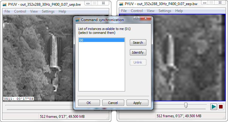
The following clips are in grayscale (B/W) colorspace, decompressed after transmission on an error prone channel, with the indicated Symbol Error Rate (SER).

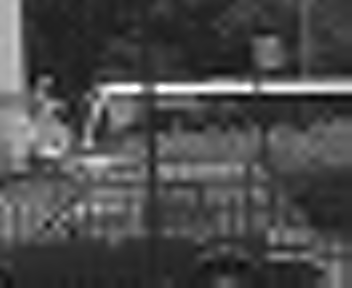

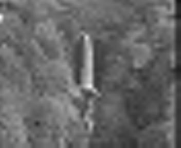
The following clips are in grayscale (B/W) colorspace, decompressed after transmission on an error prone channel, with the indicated Symbol Error Rate (SER).


The following .MAT files contain the results of the simulation described in sec. V-B.
The variables in the MAT file are:
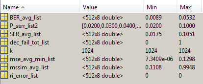
The matrixes contain the per-frame results along the rows, and different SER along the columns.
The simulated SER is contained in the
array P_serr_list2. The
measured BER and SER are in BER_avg_list and SER_avg_list.
The MSE and MSSIM are in mse_avg_min_list and mssim_avg_list.
The PSNR/MSSIM history can be plotted with
plot(0:511,
10.*log10(1./mse_avg_min_list(:,6)), 'b')
The PSNR vs. SER/BER can be plotted with
plot(mean(BER_avg_list),
10.*log10(1.0./(mean(((mse_avg_min_list))))),'bs-')
The CDF of the MSE can be obtained with
O = 10 .^ (-4:0.04:0);

[C, x] = hist(mse_avg_min_list(:, 4),
O);

C = C ./ sum(C);

C = cumsum(C);

semilogx(x, C, '-bs')
Page last modified: June 4th,
2015